* 2. Include this script: * 3. Create charts with minimal configuration - colors are auto-applied! */ (function() { 'use strict'; // ========================================================================== // READ COLORS FROM CSS CUSTOM PROPERTIES // This ensures chart colors stay in sync with the theme // ========================================================================== /** * Get a CSS custom property value from :root */ function getCSSVar(name, fallback = '') { if (typeof getComputedStyle === 'undefined') return fallback; const value = getComputedStyle(document.documentElement).getPropertyValue(name).trim(); return value || fallback; } /** * Build palette from CSS custom properties (with fallbacks) */ function buildPaletteFromCSS() { return { // Primary brand colors dartmouthGreen: getCSSVar('--dartmouth-green', '#00693e'), textPrimary: getCSSVar('--text-primary', '#0a2518'), textSecondary: getCSSVar('--text-secondary', '#0a3d23'), // Chart colors (from CSS --chart-color-N variables) chartColors: [ getCSSVar('--chart-color-1', '#00693e'), getCSSVar('--chart-color-2', '#267aba'), getCSSVar('--chart-color-3', '#ffa00f'), getCSSVar('--chart-color-4', '#9d162e'), getCSSVar('--chart-color-5', '#8a6996'), getCSSVar('--chart-color-6', '#a5d75f'), getCSSVar('--chart-color-7', '#003c73'), getCSSVar('--chart-color-8', '#d94415'), getCSSVar('--chart-color-9', '#643c20'), getCSSVar('--chart-color-10', '#c4dd88'), getCSSVar('--chart-color-11', '#f5dc69'), getCSSVar('--chart-color-12', '#424141'), ], // Background colors (semi-transparent versions) chartBgColors: [ getCSSVar('--chart-bg-1', 'rgba(0, 105, 62, 0.5)'), getCSSVar('--chart-bg-2', 'rgba(38, 122, 186, 0.5)'), getCSSVar('--chart-bg-3', 'rgba(255, 160, 15, 0.5)'), getCSSVar('--chart-bg-4', 'rgba(157, 22, 46, 0.5)'), getCSSVar('--chart-bg-5', 'rgba(138, 105, 150, 0.5)'), getCSSVar('--chart-bg-6', 'rgba(165, 215, 95, 0.5)'), ], // Semantic colors positive: getCSSVar('--chart-positive', '#00693e'), negative: getCSSVar('--chart-negative', '#9d162e'), neutral: getCSSVar('--chart-neutral', '#424141'), highlight: getCSSVar('--chart-highlight', '#ffa00f'), // Grid and axis colors gridLight: getCSSVar('--chart-grid-light', 'rgba(0, 105, 62, 0.1)'), gridMedium: getCSSVar('--chart-grid-medium', 'rgba(0, 105, 62, 0.15)'), gridDark: getCSSVar('--chart-grid-dark', 'rgba(0, 105, 62, 0.2)'), axisColor: getCSSVar('--chart-axis-color', '#0a2518'), // Font fontFamily: getCSSVar('--chart-font-family', "'Avenir LT Std', 'Avenir', 'Avenir Next', -apple-system, BlinkMacSystemFont, sans-serif"), }; } // Initialize palette (will be populated when DOM is ready) let CDL_PALETTE = null; // For convenience, expose primary chart colors array let CHART_COLORS = null; // ========================================================================== // FONT CONFIGURATION // Responsive font sizes based on typical Marp slide dimensions (1280x720) // ========================================================================== const FONT_CONFIG = { sizes: { title: 22, // Chart title subtitle: 18, // Subtitle legend: 16, // Legend labels axisTitle: 18, // Axis titles axisTicks: 16, // Axis tick labels tooltip: 14, // Tooltip text dataLabels: 14, // Data labels on charts }, weight: { normal: 400, medium: 500, bold: 600, }, }; // ========================================================================== // HELPER FUNCTIONS // ========================================================================== /** * Ensure palette is initialized */ function ensurePalette() { if (!CDL_PALETTE) { CDL_PALETTE = buildPaletteFromCSS(); CHART_COLORS = CDL_PALETTE.chartColors; } return CDL_PALETTE; } /** * Get color for a dataset at given index * Cycles through palette if more datasets than colors */ function getColor(index) { ensurePalette(); return CHART_COLORS[index % CHART_COLORS.length]; } /** * Get color with alpha transparency */ function getColorWithAlpha(color, alpha) { // Handle hex colors if (color.startsWith('#')) { const r = parseInt(color.slice(1, 3), 16); const g = parseInt(color.slice(3, 5), 16); const b = parseInt(color.slice(5, 7), 16); return `rgba(${r}, ${g}, ${b}, ${alpha})`; } // Handle rgba colors if (color.startsWith('rgba')) { return color.replace(/[\d.]+\)$/, `${alpha})`); } return color; } /** * Generate colors for all datasets in chart data * Automatically assigns colors if not specified */ function autoAssignColors(data, chartType) { if (!data || !data.datasets) return data; data.datasets.forEach((dataset, index) => { const baseColor = getColor(index); // Only assign colors if not already specified switch (chartType) { case 'bar': case 'horizontalBar': if (!dataset.backgroundColor) { dataset.backgroundColor = baseColor; } if (!dataset.borderColor) { dataset.borderColor = baseColor; } if (dataset.borderWidth === undefined) { dataset.borderWidth = 2; } break; case 'line': if (!dataset.borderColor) { dataset.borderColor = baseColor; } if (!dataset.backgroundColor) { dataset.backgroundColor = getColorWithAlpha(baseColor, 0.1); } if (dataset.borderWidth === undefined) { dataset.borderWidth = 3; } if (dataset.pointRadius === undefined) { dataset.pointRadius = 6; } if (!dataset.pointBackgroundColor) { dataset.pointBackgroundColor = baseColor; } if (dataset.tension === undefined) { dataset.tension = 0.3; } break; case 'scatter': case 'bubble': if (!dataset.backgroundColor) { dataset.backgroundColor = baseColor; } if (!dataset.borderColor) { dataset.borderColor = baseColor; } if (dataset.pointRadius === undefined) { dataset.pointRadius = 15; } if (dataset.pointHoverRadius === undefined) { dataset.pointHoverRadius = 18; } break; case 'pie': case 'doughnut': case 'polarArea': // For pie charts, we need multiple colors for one dataset if (!dataset.backgroundColor) { const numItems = dataset.data ? dataset.data.length : 6; dataset.backgroundColor = []; for (let i = 0; i < numItems; i++) { dataset.backgroundColor.push(getColor(i)); } } if (!dataset.borderColor) { dataset.borderColor = '#d8d8d8'; // Slide background } if (dataset.borderWidth === undefined) { dataset.borderWidth = 2; } break; case 'radar': if (!dataset.borderColor) { dataset.borderColor = baseColor; } if (!dataset.backgroundColor) { dataset.backgroundColor = getColorWithAlpha(baseColor, 0.2); } if (dataset.borderWidth === undefined) { dataset.borderWidth = 2; } if (dataset.pointRadius === undefined) { dataset.pointRadius = 4; } if (!dataset.pointBackgroundColor) { dataset.pointBackgroundColor = baseColor; } break; default: // Generic color assignment if (!dataset.backgroundColor) { dataset.backgroundColor = baseColor; } if (!dataset.borderColor) { dataset.borderColor = baseColor; } } }); return data; } // ========================================================================== // CHART.JS GLOBAL DEFAULTS // ========================================================================== function applyGlobalDefaults() { if (typeof Chart === 'undefined') { console.warn('Chart.js not loaded. chart-defaults.js requires Chart.js to be loaded first.'); return false; } // Ensure palette is loaded from CSS const palette = ensurePalette(); // Font defaults Chart.defaults.font.family = palette.fontFamily; Chart.defaults.font.size = FONT_CONFIG.sizes.axisTicks; Chart.defaults.color = palette.textPrimary; // Responsive defaults Chart.defaults.responsive = true; Chart.defaults.maintainAspectRatio = false; // Animation (subtle) Chart.defaults.animation.duration = 400; // Plugin defaults // Legend Chart.defaults.plugins.legend.labels.font = { family: palette.fontFamily, size: FONT_CONFIG.sizes.legend, weight: FONT_CONFIG.weight.normal, }; Chart.defaults.plugins.legend.labels.color = palette.textPrimary; Chart.defaults.plugins.legend.labels.usePointStyle = true; Chart.defaults.plugins.legend.labels.padding = 20; // Title Chart.defaults.plugins.title.font = { family: palette.fontFamily, size: FONT_CONFIG.sizes.title, weight: FONT_CONFIG.weight.medium, }; Chart.defaults.plugins.title.color = palette.textPrimary; // Tooltip Chart.defaults.plugins.tooltip.backgroundColor = palette.textPrimary; Chart.defaults.plugins.tooltip.titleFont = { family: palette.fontFamily, size: FONT_CONFIG.sizes.tooltip, weight: FONT_CONFIG.weight.medium, }; Chart.defaults.plugins.tooltip.bodyFont = { family: palette.fontFamily, size: FONT_CONFIG.sizes.tooltip, }; Chart.defaults.plugins.tooltip.cornerRadius = 4; Chart.defaults.plugins.tooltip.padding = 10; // Scale defaults (for cartesian charts) // These need to be applied per-scale type const scaleDefaults = { grid: { color: palette.gridLight, lineWidth: 1, }, border: { color: palette.gridDark, width: 1, }, ticks: { font: { family: palette.fontFamily, size: FONT_CONFIG.sizes.axisTicks, }, color: palette.textPrimary, }, title: { font: { family: palette.fontFamily, size: FONT_CONFIG.sizes.axisTitle, weight: FONT_CONFIG.weight.normal, }, color: palette.textPrimary, }, }; // Apply scale defaults to linear scale if (Chart.defaults.scales && Chart.defaults.scales.linear) { if (Chart.defaults.scales.linear.grid) Object.assign(Chart.defaults.scales.linear.grid, scaleDefaults.grid); if (Chart.defaults.scales.linear.border) Object.assign(Chart.defaults.scales.linear.border, scaleDefaults.border); if (Chart.defaults.scales.linear.ticks) Object.assign(Chart.defaults.scales.linear.ticks, scaleDefaults.ticks); if (Chart.defaults.scales.linear.title) Object.assign(Chart.defaults.scales.linear.title, scaleDefaults.title); } // Apply scale defaults to category scale if (Chart.defaults.scales && Chart.defaults.scales.category) { if (Chart.defaults.scales.category.grid) Object.assign(Chart.defaults.scales.category.grid, scaleDefaults.grid); if (Chart.defaults.scales.category.border) Object.assign(Chart.defaults.scales.category.border, scaleDefaults.border); if (Chart.defaults.scales.category.ticks) Object.assign(Chart.defaults.scales.category.ticks, scaleDefaults.ticks); if (Chart.defaults.scales.category.title) Object.assign(Chart.defaults.scales.category.title, scaleDefaults.title); } // Apply scale defaults to logarithmic scale if (Chart.defaults.scales && Chart.defaults.scales.logarithmic) { if (Chart.defaults.scales.logarithmic.grid) Object.assign(Chart.defaults.scales.logarithmic.grid, scaleDefaults.grid); if (Chart.defaults.scales.logarithmic.border) Object.assign(Chart.defaults.scales.logarithmic.border, scaleDefaults.border); if (Chart.defaults.scales.logarithmic.ticks) Object.assign(Chart.defaults.scales.logarithmic.ticks, scaleDefaults.ticks); if (Chart.defaults.scales.logarithmic.title) Object.assign(Chart.defaults.scales.logarithmic.title, scaleDefaults.title); } // Apply scale defaults to radial scale (for radar charts) if (Chart.defaults.scales && Chart.defaults.scales.radialLinear) { if (Chart.defaults.scales.radialLinear.grid) Chart.defaults.scales.radialLinear.grid.color = palette.gridLight; if (Chart.defaults.scales.radialLinear.angleLines) Chart.defaults.scales.radialLinear.angleLines.color = palette.gridMedium; if (Chart.defaults.scales.radialLinear.pointLabels) { Chart.defaults.scales.radialLinear.pointLabels.font = { family: palette.fontFamily, size: FONT_CONFIG.sizes.axisTicks, }; Chart.defaults.scales.radialLinear.pointLabels.color = palette.textPrimary; } } return true; } // ========================================================================== // CHART WRAPPER FOR AUTO-STYLING // ========================================================================== /** * Wrap the Chart constructor to automatically apply CDL styling */ function wrapChartConstructor() { if (typeof Chart === 'undefined') return; const OriginalChart = Chart; // Create a wrapper that auto-applies colors window.Chart = function(ctx, config) { // Auto-assign colors if not specified if (config && config.data) { config.data = autoAssignColors(config.data, config.type); } // Merge default options for specific chart types if (config && config.options) { config.options = applyChartTypeDefaults(config.type, config.options); } // Call original constructor return new OriginalChart(ctx, config); }; // Copy static properties and methods Object.setPrototypeOf(window.Chart, OriginalChart); Object.assign(window.Chart, OriginalChart); // Preserve the prototype chain window.Chart.prototype = OriginalChart.prototype; } /** * Apply chart-type specific defaults */ function applyChartTypeDefaults(chartType, userOptions) { const options = { ...userOptions }; switch (chartType) { case 'bar': case 'horizontalBar': // Bar chart defaults if (!options.scales) options.scales = {}; if (!options.scales.x) options.scales.x = {}; if (!options.scales.y) options.scales.y = {}; // Hide x-axis grid for cleaner look if (options.scales.x.grid === undefined) { options.scales.x.grid = { display: false }; } break; case 'line': // Line chart defaults if (!options.interaction) { options.interaction = { intersect: false, mode: 'index' }; } break; case 'pie': case 'doughnut': // Pie/doughnut defaults if (!options.plugins) options.plugins = {}; if (options.plugins.legend === undefined) { const palette = ensurePalette(); options.plugins.legend = { position: 'right', labels: { font: { family: palette.fontFamily, size: FONT_CONFIG.sizes.legend, }, color: palette.textPrimary, padding: 15, }, }; } break; case 'radar': // Radar chart defaults - keep as-is, scale defaults applied globally break; case 'scatter': case 'bubble': // Scatter/bubble defaults if (!options.scales) options.scales = {}; if (!options.scales.x) options.scales.x = {}; if (!options.scales.y) options.scales.y = {}; break; } return options; } // ========================================================================== // CONVENIENCE FUNCTIONS FOR USERS // Exposed on window.CDLChart for easy access // ========================================================================== window.CDLChart = { // Color palette access (getters to ensure lazy initialization) get colors() { return ensurePalette().chartColors; }, get palette() { return ensurePalette(); }, // Get specific color by index getColor: getColor, // Get color with transparency getColorWithAlpha: getColorWithAlpha, // Get array of colors for a specific count getColors: function(count) { ensurePalette(); const result = []; for (let i = 0; i < count; i++) { result.push(getColor(i)); } return result; }, // Font configuration fonts: FONT_CONFIG, // Quick chart creation helpers // These create minimal config that auto-applies all styling /** * Create a simple bar chart * @param {string} canvasId - Canvas element ID * @param {string[]} labels - X-axis labels * @param {number[]} data - Data values * @param {object} options - Optional overrides */ bar: function(canvasId, labels, data, options = {}) { return new Chart(document.getElementById(canvasId), { type: 'bar', data: { labels: labels, datasets: [{ data: data }], }, options: { plugins: { legend: { display: false } }, ...options, }, }); }, /** * Create a simple line chart * @param {string} canvasId - Canvas element ID * @param {string[]} labels - X-axis labels * @param {Array} datasets - Array of {label, data} objects * @param {object} options - Optional overrides */ line: function(canvasId, labels, datasets, options = {}) { return new Chart(document.getElementById(canvasId), { type: 'line', data: { labels: labels, datasets: datasets.map(ds => ({ label: ds.label, data: ds.data, fill: ds.fill !== undefined ? ds.fill : true, })), }, options: options, }); }, /** * Create a simple pie chart * @param {string} canvasId - Canvas element ID * @param {string[]} labels - Slice labels * @param {number[]} data - Data values * @param {object} options - Optional overrides */ pie: function(canvasId, labels, data, options = {}) { return new Chart(document.getElementById(canvasId), { type: 'pie', data: { labels: labels, datasets: [{ data: data }], }, options: options, }); }, /** * Create a simple scatter chart * @param {string} canvasId - Canvas element ID * @param {Array} datasets - Array of {label, data: [{x, y}]} objects * @param {object} options - Optional overrides */ scatter: function(canvasId, datasets, options = {}) { return new Chart(document.getElementById(canvasId), { type: 'scatter', data: { datasets: datasets.map(ds => ({ label: ds.label, data: ds.data, })), }, options: options, }); }, /** * Create a doughnut chart * @param {string} canvasId - Canvas element ID * @param {string[]} labels - Slice labels * @param {number[]} data - Data values * @param {object} options - Optional overrides */ doughnut: function(canvasId, labels, data, options = {}) { return new Chart(document.getElementById(canvasId), { type: 'doughnut', data: { labels: labels, datasets: [{ data: data }], }, options: options, }); }, /** * Create a radar chart * @param {string} canvasId - Canvas element ID * @param {string[]} labels - Axis labels * @param {Array} datasets - Array of {label, data} objects * @param {object} options - Optional overrides */ radar: function(canvasId, labels, datasets, options = {}) { return new Chart(document.getElementById(canvasId), { type: 'radar', data: { labels: labels, datasets: datasets.map(ds => ({ label: ds.label, data: ds.data, })), }, options: options, }); }, }; // ========================================================================== // INITIALIZATION // ========================================================================== function initialize() { // Wait for Chart.js to be available if (typeof Chart !== 'undefined') { applyGlobalDefaults(); wrapChartConstructor(); console.log('CDL Chart defaults applied successfully.'); return true; } else { // Chart.js not yet loaded - wait and retry let retries = 0; const maxRetries = 50; // 5 seconds max wait const checkInterval = setInterval(function() { retries++; if (typeof Chart !== 'undefined') { clearInterval(checkInterval); applyGlobalDefaults(); wrapChartConstructor(); console.log('CDL Chart defaults applied successfully (after waiting for Chart.js).'); } else if (retries >= maxRetries) { clearInterval(checkInterval); console.warn('Chart.js not found after waiting. CDL Chart defaults not applied.'); } }, 100); return false; } } // Initialize IMMEDIATELY - this must run BEFORE any chart creation scripts // Chart.js CDN should be loaded before this script initialize(); })();

Lecture 15: The transformer model

PSYC 51.17: Models of language and communication

Jeremy R. Manning
Dartmouth College
Winter 2026

Learning objectives

  1. Understand the transformer as a function that predicts the next word
  2. Follow data from raw text through tokenization, embedding, and attention
  3. Explain how queries, keys, and values enable self-attention
  4. See how multiple attention heads capture different patterns
  5. Understand how stacking blocks creates deep representations

The transformer model

See The Animated Transformer for a visual walkthrough of the transformer architecture. (Today's lecture is heavily inspired by this resource!)

The transformer is a machine learning model for sequence modeling. Given a sequence of things, the model can predict what the next thing in the sequence might be.

We can think of the transformer as a function: Transformer(X,θ)Y\text{Transformer}(X, \theta) \rightarrow Y

  • XX is our input sequence
  • θ\theta represents the model parameters
  • YY is the predicted next token

The transformer model

Tokenization

The transformer operates on sequences of numbers. So first we need to tokenize the input text into discrete units (tokens) and map those tokens to unique IDs. The model doesn't understand tokens directly—it identifies them using unique numbers from a vocabulary.

"the robots will bring" → [3206, 2736, 3657, 400]

Each word maps to a unique ID in the vocabulary. (In practice, tokenization is more complex—subword units, punctuation, etc.—but this simplified example suffices for our purposes.)

Embeddings: numbers speak louder than words

The transformer maintains embeddings of each token in its vocabulary. These embeddings are learned vectors that capture semantic information about the tokens.

This is the same idea as LSA, LDA, Word2Vec, GloVe, FastText, etc.- but here the embeddings are learned jointly with the rest of the model.

Token embeddings

Token embeddings

Our transformer has embedding vectors of length C=768C = 768. All embeddings can be packed together in a single T×CT \times C matrix, where (in our example) T=4T = 4 is the number of input tokens.

Each row of this matrix corresponds to a token in the input sequence, and each column corresponds to a dimension in the embedding space.

Position embeddings

Position embeddings

Each position in the input sequence (1st, 2nd, 3rd, etc.) also has a learned embedding vector of length C=768C = 768. These position embeddings are stored in a separate T×CT \times C matrix.

In order to capture the significance of the position of a token within a sequence, the transformer also maintains embeddings for each position.

Without position information, "cat sat" and "sat cat" would look identical to the model!

Each row of this matrix corresponds to a position in the input sequence, and each column corresponds to a dimension in the embedding space.

Notice that both token and position embeddings have the same shape: T×CT \times C. This allows the model to capture both the identity of the token and its position in the sequence within compatable embedding spaces.

Combined embeddings

Combined embeddings

The token and position embedding matrices (T×CT \times C each) are added together to obtain a position-dependent embedding for each token.

The token and position embeddings are all part of θ\theta, meaning they are tuned during model training.

Adding the embeddings allows the model to consider both the identity of the token and its position in the sequence simultaneously.

Queries, keys, and values

The Transformer computes three vectors for each token: query, key, and value. This is done by multiplying with learned weight matrices:

Q=XWQK=XWKV=XWVQ = XW_Q \quad K = XW_K \quad V = XW_V

The weight matrices WQW_Q, WKW_K, WVW_V are all part of θ\theta.

The WQW_Q, WKW_K, and WVW_V matrices each have shape C×CC \times C. Multiplying the input matrix XX (T×CT \times C) by these weight matrices results in three new T×CT \times C matrices: QQ, KK, and VV.

Queries, keys, and values

Queries, keys, and values

Imagine you have a database of images with text descriptions:

  • Query: the user's search text
  • Key: the text descriptions in your database
  • Value: the actual images

Only those images (values) whose descriptions (keys) best match the search (query) are returned.

Self-attention works similarly—tokens "query" other tokens to find which ones they should "pay attention" to. In this context, "paying attention" means incorporating information from relevant tokens into their own representation (i.e., their row in the output matrix).

Many heads are better than one

The Transformer splits the Q, K, V matrices into multiple heads. With C=768C = 768 columns and 12 heads, each head operates on 64 dimensions.

Different heads can specialize in different patterns: syntax, co-reference, semantic roles, etc. The model "decides" (i.e., learns from training data) what's useful!

Splitting into heads

Time to pay attention

Self-attention is the core idea behind the transformer. We compute an attention scores matrix:

A=QKTHA = \frac{Q \cdot K^T}{\sqrt{H}}

This matrix tells us how much attention each token should pay to every other token.

  • QQ is T×CT \times C
  • KTK^T is C×TC \times T
  • AA is T×TT \times T
  • HH is the head dimension (e.g., 64)
  1. AA can be enormous for long sequences (e.g., 20482048 tokens → 2048×20482048 \times 2048 matrix). This is a key computational bottleneck.
  2. Notice that the "VV" matrix isn't used yet; it'll come back soon!

Computing attention scores

Applying attention

The attention score for a token needs to be masked if it occurs later in the sequence. In our example, "bring" can pay attention to "robots", but not vice-versa—a token shouldn't look at future tokens when predicting its next token.

To get the final output, we need to apply the attention scores to the value matrix VV by multiplying AA and VV.

VV contains the information we want to aggregate, while AA tells us how much of each token's value to include in the output for each token. We end up with a new T×CT \times C matrix where each token's representation is a weighted sum of the value vectors of all tokens.

  1. Mask future tokens (set upper triangle to -\infty)
  2. Softmax each row (normalize to probabilities)
  3. Multiply by V (weighted sum of value vectors)

The softmax function converts raw scores into probabilities (note: -\infty becomes 0 after softmax):

softmax(zi)=ezijezj\text{softmax}(z_i) = \frac{e^{z_i}}{\sum_{j} e^{z_j}}

Applying attention

Merging heads

After computing attention outputs for each head, we concatenate the outputs from all heads along the feature dimension to form a single T×CT \times C matrix.

Each head captures different aspects of the input sequence. By concatenating them, we preserve the diverse information learned by each head.

Remember how in ELIZA our text processing function computed the output (response) by combining various features of the input? The effect of applying attention and merging heads is similar: we get a rich representation of the input sequence that informs us about future tokens. This will be used in the next step to make predictions about the next token in the sequence.

The effect of adding in positional information and applying attention is that each token's representation now encodes not just its identity, but also its context within the sequence. This "sneaks in" more learnable parameters that enable the model to capture rich temporal structure in the data.

Merging heads

Feed forward

A feed-forward network processes each token's representation independently using two linear transformations with a non-linear activation in between:

FFN(x)=ReLU(xWnn+b1)Wmm+b2\text{FFN}(x) = \text{ReLU}(xW_{nn} + b_1)W_{mm} + b_2

The hidden layer expands to 4C=30724C = 3072 dimensions, then projects back to C=768C = 768.

  • WnnW_{nn}: C×4CC \times 4C
  • b1b_1: 4C4C (gets replicated for each token; not shown in next animation)
  • WmmW_{mm}: 4C×C4C \times C
  • b2b_2: CC (gets replicated for each token; not shown in next animation)

Everything so far has used linear operations. The non-linearity (ReLU) in the FFN allows the model to learn complex, non-linear relationships.

Feed-forward network

Feed-forward network

All the weight matrices in the FFN are part of θ\theta (i.e., the model parameters) and are learned during training. The FFN allows the model to transform the attention outputs into richer representations before passing them to the next layer.

The expansion to 4C4C dimensions allows the model to capture more complex patterns, while the projection back to CC ensures that the output remains compatible with the rest of the model.

We need to go deeper

All the steps thus constitute a single transformer block. Each block takes a T×CT \times C matrix as input and outputs a T×CT \times C matrix.

  • GPT-2: 12–48 blocks
  • GPT-3: 96 blocks
  • GPT-4+: 100+ blocks (exact architecture not public)

Stacking transformer blocks

Making a prediction

Take the last token's output vector (1×C1 \times C) and multiply by a C×VC \times V weight matrix, where VV is the vocabulary size. Normalize (softmax) to get a probability distribution over all words.

In our example, "prosperity" might get a 92% probability, but "suffering" only 20%, and so on.

So if "prosperity" has the highest probability, the model predicts "the robots will bring prosperity"

We only care about predicting the next token after the entire input sequence, so we only use the output corresponding to the last token. But we needed to process the entire sequence to get context!

Making a prediction

Text generator go brrr
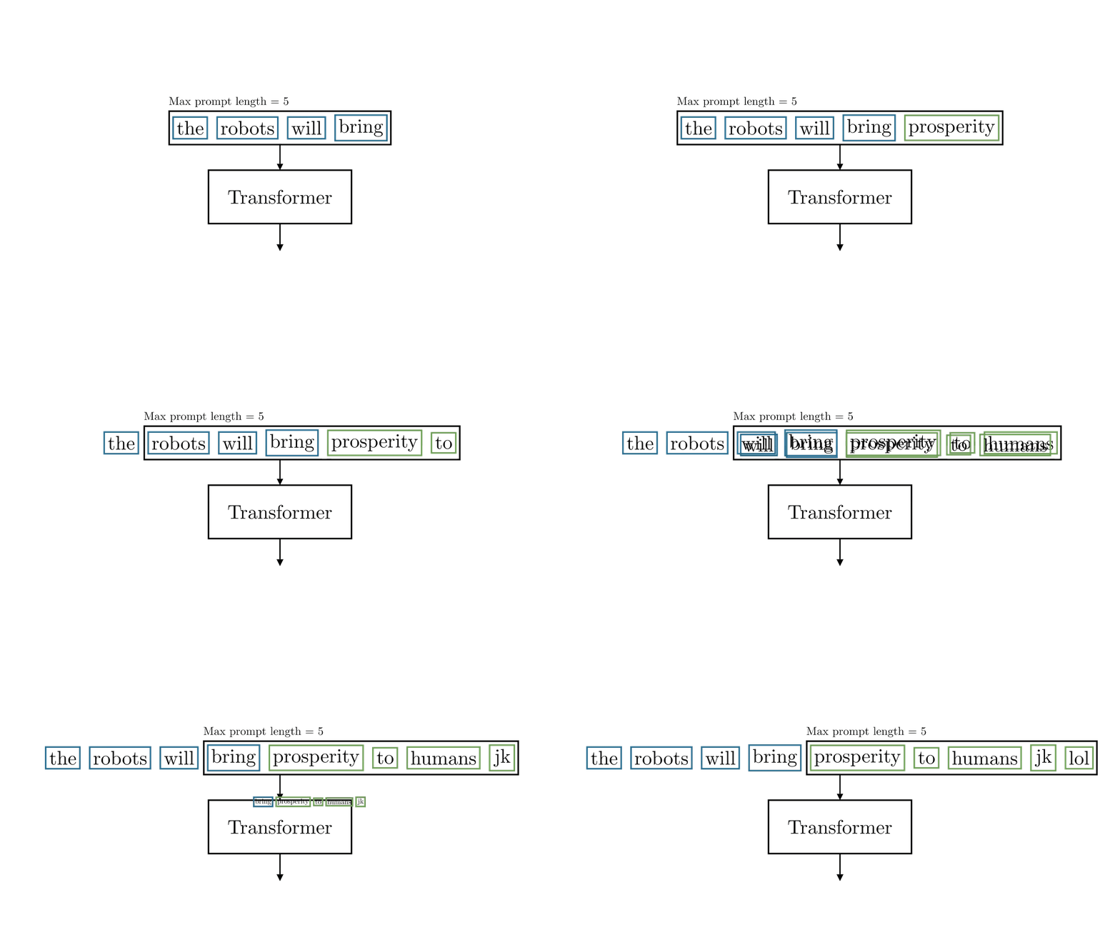
Autoregressive generation

The first token produced is added to the prompt and fed back to produce the second token, which is then fed back to produce the third, and so on.

Transformers have a maximum context length (N tokens). As generation continues, we drop the oldest tokens.

Remember that AA matrix? Its size grows quadratically with context length (N×NN \times N). Longer contexts require more memory and computation, which can be a bottleneck. This limits how far back the model can "remember" during generation: tokens prior to the start of the context window are completely invisible to the model!

And...that's it!

  1. Tokenize text to IDs
  2. Embed tokens + positions
  3. Project to Q, K, V
  4. Split into attention heads
  5. Compute attention scores
  6. Apply masking and softmax
  7. Multiply by V for output
  8. Feed forward with non-linearity
  9. Stack many blocks
  10. Predict next token

...Mostly!

To focus on the most important aspects, we skipped:

  • Layer normalization (stabilizes training)
  • Residual connections (helps gradient flow)
  • Dropout (regularization)
  • Training (how θ\theta is learned)

See nanoGPT for a complete implementation.

References

Vaswani et al. (2017, arXiv) "Attention Is All You Need" — The original transformer paper.

The Animated Transformer — Visual walkthrough that inspired this lecture.

The Illustrated Transformer — Jay Alammar's detailed visual guide.

nanoGPT — Andrej Karpathy's minimal GPT implementation.

Questions?

📧 Email
💬 Discord

Training transformers: where do the parameters (θ\theta) come from?